The Symmetric gradient: an odd 40 year curiosity in matrix algebra

There shouldn’t be anything particularly difficult about differentiating with respect to symmetric matrices.

Differentiation is defined over abstract spaces. And the set of real symmetric matrices $\mathbb{S}_n(\mathbb{R})$ is not special. And yet, this past semester, Paul and I, along with a student, Aleksandr, ran into problems.

It turns out that this problem of computing gradients with respect to a symmetric matrix is common enough that several confusing threads on mathoverflow on the topic exist. Each proposing slightly different solutions, with some, surprisingly, arguing that gradients of scalar functions of symmetric matrices aren’t well defined.

This doesn’t make sense. Again, there shouldn’t be anything fancy required for computing gradients of symmetric matrices. Luckily for us, Shriram Srinivasan and Nishant Panda¹ pinpointed the root of the confusion: there were some imprecisions early in the litterature² on the topic about what exactly we mean by gradient. This is led to the appearance of odd formulas making obscure what should be simple.

At the heart of the confusion is the question:

Is the gradient the vector of partial derivatives or 
is it the Riesz representant of the Jacobian ?

What follows is a dramatic retelling of our story with jax, the symmetric gradient and how to adapt the results in ¹ for hessians.

The hessian of a strongly convex function#

Consider the strongly convex function $f$ over the set of real symmetric matrices defined as

$$f:\begin{cases} \mathbb{S}_n(\mathbb{R}) \rightarrow \mathbb{R} \\ X \mapsto -\frac{1}{2}\left(\log(\det( I - X)) + \log(\det( I + X))\right) \end{cases}$$

The strong convexity of $f$ implies that the hessian of $f$ should define a positive definite quadratic form. Since $f$ is a function taking as input $n\times n$ matrices, we expect, the hessian $\nabla^2 f$ to be an $n\times n \times n \times n$ monstrosity. Luckily automatic differentiation exists, so we can feed this function to jax’s automatic differatiation engine, it will compute the hessian for us :

from jax import grad, jacobian
import jax.numpy as jnp

def f(X):
    A = jnp.identity(2) - X
    B = jnp.identity(2) + X
    return -0.5*(jnp.linalg.slogdet(A)[1] + jnp.linalg.slogdet(B)[1])
    

tensorHess = jacobian(grad(f))

According to jax documentation, the returned objecttensorHess is the $n\times n \times n \times n$ tensor whose coordinates are $$ \text{tensorHess}_{i, j, k, l} = \frac{\partial f}{\partial x_{k,l} \partial x_{i,j}}, $$

for any $0 \leq i,j,k,l \leq n-1$ (using zero-indexing as God intended) .

In order to check that this hessian is indeed positive definite as theory predicts, we can first write it in matrix form, then, compute its eigenvalues to confirm that it is indeed positive definite.

The tensor tensorHessis just linear map from $\mathbb{R}^{n \times n}$ to $\mathbb{R}^{n \times n}$, so we can write it as a linear map from $\mathbb{R}^{n^2}$ to $\mathbb{R}^{n^2}$ as long as we define a vectorization (or flattening) of the elements of $\mathbb{R}^{n \times n}$.

A straightforward flattening of matrices $\text{vec} : \mathbb{R}^{n \times n} \rightarrow \mathbb{R}^{n^2}$ can be obtained by chaining the rows next to each other and transposing to obtain a vector in $\mathbb{R}^{n^2}$. In python, this flattening would correspond to the function

def vec(M):
    flattened = np.zeros(n*n)
    for i in range(n):
        for j in range(n):
            flattened[i*n + j] = M[i, j]
    return flattened

The corresponding reverse operation $\text{mat} : \mathbb{R}^{n^2} \rightarrow \mathbb{R}^{n\times n}$ can easily be derived by dividing the vector into chunks of size $n$ and stacking the chunks into rows. It turns out that these operations are exactly what numpy’s reshape function does !

With this flattening in hand, we can write the matrix version $M_{hess}$ of tensorHess by using the definition of the partial derivative, i.e the fact that

$$\text{vec}(E_{k,l})^TM_{hess}\text{vec}(E_{i,j}) = \frac{\partial f}{\partial x_{k,l} \partial x_{i,j}} =\text{tensorHess}_{i, j, k, l}.$$

Now since $\text{vec}(E_{i,j})$ is a vector with a single $1$ at the $i\times n + j$ coordinate, we find that

$$[M_{hess}]_{p, q} = \text{tensorHess}_{\lfloor \frac{p}{n} \rfloor, \; p\;\mathbf{ mod }\; n, \lfloor \frac{q}{n} \rfloor, \; q;\mathbf{ mod }\; n\;}.$$

In python, this would yield the following matrixify function :

def matrixify(tensor):
    mat = np.zeros((n*n, n*n))
    for i in range(n):
        for j in range(n):
            for k in range(n):
                for l in range(n):
                    mat[j*n + i, l*n+k] = tensor[i, j, k, l]
    return mat

This, luckily for us, is again the exact procedure used by default in numpy’s reshape function ! We can finally test if, as theory predicts, the hessian is positive definite by computing its eigenvalues.

Testing positive definiteness#

In order to test that $f$ is positive definite. We pick a random point within the domain of $f$ and compute the eigenvalues of the hessian at that point :

#Picking a random point within the domain of f
test_point = np.random.randn(n, n)
test_point = 0.5 * (test.T + test)
spec_nrm = np.linalg.norm(test, ord=2)
test_point = 0.7/spec_nrm * test_point

#Computing the hessian
matHess = tensorHess(test_point).reshape(n*n, n*n)

print(np.linalg.eigvalsh(matHess))

[-2.1573663  1.0445824  2.1573663  5.728565 ]

There’s a negative eigenvalue appearing ! What went wrong ?? Let us look at the eigenvector corresponding to the negative eigenvalue.

eigvals, eigvecs = np.linalg.eigh(matHess)

for i in range(len(eigvals)):
    if eigvals[i] < 0:
        print(eigvecs[:, i].reshape(n, n))

        #Test if it is symmetric 
        print(eigvecs[:, i].reshape(n, n) == eigvecs[:, i].reshape(n, n).T)

The eigenvector (or flattened eigenmatrix to be precise) is NOT a symmetric matrix. It corresponds to wiggling the function at test_point along a non-symmetric direction.

Our function being defined over symmetric matrices, all the considered directions when computing differentials should be symmetric. So the existence of this negative eigenvalue is not proof of a mistake in convexity theory. But rather, it show us that there might be an issue coming from our interpretation of the automatic differentiation procedure.

Remember that from jax’s point of view, the symmetry constraint on the coefficients of the input does not exist. jax computes the partial derivatives as if we could move each coordinate independently of one another. The hessian computed by jax is therefore “too big” in some sense, it contains information along too many directions, some of which are not allowed.

In other words, jax isn’t computing the hessian of $f$ but the hessian of

$$g: \begin{cases} {\mathbb{R}^{n\times n}} \rightarrow \mathbb{R} \\ X \mapsto -\frac{1}{2}\left(\log(\det( I - X)) + \log(\det( I + X))\right) \end{cases}$$

a function over ${\mathbb{R}^{n\times n}}$ that, when restricted to $\mathbb{S}_n(\mathbb{R})$ gives $f$. So how can we relate the “larger” jacobians $J_{\nabla g}$ and $J_g$ to $J_{\nabla f}$ and $J_f$ ?

Going from a differential over $\mathbb{R}^{n\times n}$ to a differential over $\mathbb{S}_n(\mathbb{R})$.#

This is the question that led to various odd results in matrix algebra. If we look it up in the matrix cookbook, we find the following:

If we translate it to our setting, it would mean $$\nabla f = \nabla g + (\nabla g)^T - \text{diag}(\nabla g).$$ This results contradicts what we would find by simply looking at the definition of jacobians. Recall that the jacobian of g, denoted $J_g$, is the unique linear map from $\mathbb{R}^{n\times n}$ to $\mathbb{R}$ such that for all $X \in \mathbb{R}^{n\times n}$,

$$g(X + H) - g(X) = J_{g(X)}(H) + o( \| H\|),$$

for any $H \in \mathbb{R}^{n\times n}$. In particular this implies that, when we restrict to symmetric $X$ and $H$, we have

$$f(X + H) - f(X) = J_{g(X)}(H) + o( \| H\|).$$

So by unicity of the linear map we conclude that $J_f = J_{g|\mathbb{S}_n(\mathbb{R})}$, i.e., $J_f$ is just the restriction of $J_g$ to $\mathbb{S}_n(\mathbb{R})$. Writing restriction of domains as projections of the input variable, we can write

$$J_f \circ \text{sym} = J_{g|\mathbb{S}_n(\mathbb{R})} = J_g \circ \text{sym},$$

where $\text{sym}$ is the orthogonal projection onto $\mathbb{S}_n(\mathbb{R})$ given by $\text{sym}(M) = \frac{1}{2}\left( M + M^T\right)$. Transposing to obtain the gradient we find

$$\text{sym}(\nabla f) = \text{sym} (\nabla g) \implies \nabla f = \text{sym} (\nabla g),$$

since orthgonal projections are self-adjoint. Similarly for the hessians, we obtain

$$\text{sym} \circ J_{\nabla f} \circ \text{sym} = \text{sym} \circ J_{\nabla g} \circ \text{sym} \implies J_{\nabla f} \circ \text{sym} = \text{sym} \circ J_{\nabla g} \circ \text{sym}.$$

The relationships between differentials over $\mathbb{R}^{n\times n}$ with differentials over $\mathbb{S}_n(\mathbb{R})$ is therefore a simple intuitive relation that comes from restricting the domain of the larger differential.

A simple projection gives the symmetric gradient, not some odd formula treating the diagonal differently.

With this knowledge in hand, we can obtain the eigenvalues of the hessian of $f$ by computing the eigenvalues of

$$\text{matrixify}(\text{sym}) \cdot \text{matrixify}(\text{tensorHess}) \cdot \text{matrixify}(\text{sym}).$$

By simply excluding the zero eigenvalues coming from non-symmetric eigenvectors, we can obtain the eigenvalues of the hessian. But this exclusion of eigenvalues requires us to check the associated eigenvectors to do the elimination procedure. It turns out there is another way that doesn’t involve costly eliminations.

There are only $m = \frac{n(n+1)}{2}$ effectively free variables because of the symmetry constraint, so why not reduce the hessian into a hessian in this smaller space ? We can then compute the eigenvalues in a more direct fashion.

A derivative in the right space#

In order to derive a procedure to “reduce” the jax hessian, we need to first define a two essential linear operators. Let $P \in \mathbb{R}^{m \times n^2}$ be the matrix that, given a flattened symmetric matrix, strips away duplicate entries in such that

$$\forall M \in \mathbb{S}_n(\mathbb{R}), \; v = P\text{vec}(M) \in \mathbb{R}^m.$$

And let $D \in \mathbb{R}^{n^2 \times m}$ be the inverse operation that duplicates the entries of a vector in $\mathbb{R}^m$ so that it corresponds to the flattening in $\mathbb{R}^{n^2}$ of a symmetric matrix: $$\forall v \in \mathbb{R}^m, M = \text{mat}(Dv) \in \mathbb{S}_n(\mathbb{R}).$$

With $P$ and $D$ in hand, the space $\mathbb{S}_n(\mathbb{R})$ of dimension $m = \frac{n(n+1)}{2}$ can be identified with the space $\mathbb{R}^m$ since we can associate each symmetric matrix $M$ to a vector $v_M \in \mathbb{R}^m$ and vice versa.

Now comes the subtle point : let us compare the inner products in the original space $\mathbb{S}_n(\mathbb{R})$ with the inner products after the embedding:

$$\begin{aligned} \forall M, N\in \mathbb{S}_n(\mathbb{R}), \; \; \; \langle M, N \rangle_F & = \langle \text{mat}(Dv_M) , \text{mat}(Dv_N) \rangle_F \\ &= \langle Dv_M , Dv_N \rangle_{\mathbb{R}^{n^2}} \\ & = \langle D^TD v_M, v_N \rangle_{\mathbb{R}^{m}} \\ & {\neq \langle v_M, v_N \rangle_{\mathbb{R}^{m}}}\end{aligned}$$

We therefore cannot take the canonical inner product in $\mathbb{R}^m$ if we wish to have an embedding that preserves inner products and norms. The isometric embedding we choose to work in is the one that associates a symmetric matrix $M$ to a vector $v_m$ in the space $(\mathbb{R}^m, \langle \cdot, \cdot \rangle_{D})$ where the inner product is defined as

$$\forall u, v \in \mathbb{R}^m, \langle u, v \rangle_D = \langle D^TD u, v \rangle_{\mathbb{R}^{m}}.$$

Going back to our function $f$, if we take note of the symmetry constraints in the domain, we can see that $f : \mathbb{S}_n(\mathbb{R}) \rightarrow \mathbb{R}$ can be identified with a function $\bar{f}: \mathbb{R}^m \rightarrow \mathbb{R}$ where

$$\bar{f}(x) = g(\text{mat}(Dx))$$

With the chain rule, we can compute the Jacobian of $\bar{f}$. We find that

$$J_{\bar{f}} (x) = J_g(\text{mat}(Dx)) \circ J_\text{mat}(Dx) \circ J_D(x) = J_g(\text{mat}(Dx)) \circ \text{mat} \circ D.$$

The Jacobian we have just obtained is a linear map from $(\mathbb{R}^m, \langle \cdot, \cdot \rangle_{D})$ to $\mathbb{R}$. Had the inner product in $\mathbb{R}^m$ been the canonical one, we would have obtained the gradient by simply transposing. In our case however, we have to put in some some work. The gradient is the Riesz representant of the Jacobian, and when the inner product is exotic, simply transposing won’t do. With a few simple manipulations left for the appendix, we find that

$$\nabla \bar{f}(x) = (\text{mat} \circ D)^T \circ \nabla g(\text{mat}(Dx)) = P \circ \text{vec} \circ \nabla g(\text{mat}(Dx))$$

To obtain the hessian, we can again compute the jacobian of the gradient using the chain rule, we find that

$$\nabla^2 \bar{f}(x) = P \circ \text{vec} \circ J_{\nabla g}(\text{mat}(Dx)) \circ \text{mat} \circ D = P \circ \text{matrixify}(J_{\nabla g}(\text{mat}(Dx))) \circ D$$

Here we used the fact that, by definition of the matrixification procedure, $\text{vec} \circ J_{\nabla g}(\text{mat}(Dx)) \circ \text{mat} = \text{matrixify}(J_{\nabla g}(\text{mat}(Dx)))$.

We have our reduction ! We simply apply $P$ and $D$ to matHess and it will give us $\nabla^2 \bar{f}$ which, by strong convexity of $\bar{f}$, is certainly positive definite because in$(\mathbb{R}^m, \langle \cdot, \cdot \rangle_{D})$, we do not exclude any directions.

But wait how would we compute eigenvalues of a linear map acting in $(\mathbb{R}^m, \langle \cdot, \cdot \rangle_{D})$ ?

Relating the eigenvalues of the smaller hessian and the jax hessian#

Let $\lambda$ be an eigenvalue of matHess at $x$ with associated symmetric eigenvector $M=\text{mat}(Dv)$. Then,

$$ \begin{aligned} \nabla^2 \bar{f}(x) v &= P \circ \text{matrixify}(J_{\nabla g}(\text{mat}(Dx))) \circ D v \\
&= P (\lambda \cdot Dv) \\
&= \lambda PD v \\
&= \lambda v. \end{aligned} $$ Any eigenvalue of matHess corresponding to a symmetric eigenvector is also an eigenvalue of $\nabla^2 \bar{f}(x)$. Reciprocally, if $\lambda$ is an eigenvalue of $\nabla^2 \bar{f}(x)$ with associated eigenvector $v$, then, $$ \begin{aligned} \lambda v &= \nabla^2 \bar{f}(x) v = P \circ \text{matrixify}(J_{\nabla g}(\text{mat}(Dx))) \circ D v \\
\lambda v &= P \text{matHess(x)}Dv \\
\lambda D v &= DP \text{matHess(x)} Dv\\
\lambda D v &= \text{matHess(x)} Dv. \end{aligned} $$ The eigenvalues of $\nabla^2 \bar{f}(x)$ entirely capture the behavior of matHess when restricted to symmetric matrices. Now all we need is a way to compute them.

Since we are living in a space with an exotic inner product, the vanilla eigh function of numpy/scipy won’t do. Indeed, the eigenvectors of the symmetric matrix $\nabla^2 \bar{f}(x)$ should define an orthormal basis in $(\mathbb{R}^m, \langle \cdot, \cdot \rangle_{D})$. To find them, we need to solve a generalized eigenvalue problem that computes a set of vectors ${v_1, \dots, v_m}$ such that $\nabla^2 \bar{f}(x)v_i = \lambda_i v_i$ and such that $\langle v_i, v_j \rangle_D = 0$ if $\lambda_i \neq \lambda_j$.

Solving the generalized eigenvalue problem: $$ (D^TD)\nabla^2 \bar{f}(x)v = \lambda (D^TD)v $$ yields eigenvectors with the desired property.

This problem can be solved using scipy’s generalized eigenvalue solver:

true_dim_eigvals = scipy.linalg.eigh(a=(D.T@D) @ matHess, b=(D.T@D))

So to summarize, in order to confirm what we already know, that is the fact that $f$ is strongly convex, we can use jax to compute the hessian, reduce it to the proper dimension by applying $P$ and $D$ and compute its eigenvalues by solving a generalized eigenvalue solver. With this we can show that math holds up. I have yet to see a better use of our time

Recovering the mistaken identity in matrix textbooks#

Now imagine we forget that our embedded space has an exotic inner product. We would think there is no subtelty in defining the gradient so we would take it to be the matrix of partial derivatives.

Had we made this mistake in our computation of $\nabla \bar{f}$, we would have found that

$$\nabla \bar{f}(x) = D^T \circ \text{vec} \circ \nabla g(\text{mat}(Dx)).$$

This comes as a result of taking the transpose of the Jacobian instead of its Riesz representant. With some simplification, this yields

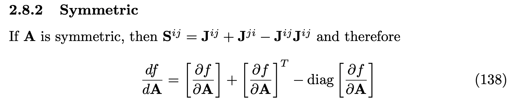
$$\nabla \bar{f}(x) = P \circ \text{vec}( \nabla g(\text{mat}(Dx)) + \nabla g(\text{mat}(Dx))^T - \text{diag}(\nabla g(\text{mat}(Dx)))).$$

We would conclude that

$$ \begin{aligned} \nabla {f}(x) &= \text{mat}(D \nabla \bar{f}(x)) \\
&= \nabla g(\text{mat}(Dx)) + \nabla g(\text{mat}(Dx))^T - \text{diag}(\nabla g(\text{mat}(Dx))), \end{aligned} $$ thus recovering the odd formula in the matrix cookbook. All this coming from our ignorance of the subtelties coming from not having the canonical inner product.

This seemingly minor distinction of whether or not the gradient corresponds to the vector of partial derivatives or the Riesz representant of the Jacobian matters. It matters especially when the gradient is used in optimization.

We can see this by trying to optimize the function $h: X \mapsto tr(X^2)$ over the set of $2\times 2$ symmetric matrices. To do so we, can identify this function $h: \mathbb{S}_n(\mathbb{R}) \to \mathbb{S}_n(\mathbb{R})$ with a function $\hat{h}: \mathbb{R}^m \to \mathbb{R}^m$ defined as $$ \hat{h} : x \mapsto tr((\text{mat}(Dx))^2). $$

Clearly, any matrix having $0$ eigenvalues is in the argmin and from any initialization, the fastest way to get from the initial eigenvalues to $0$ is to go in a straight line in the space of eigenvalues. We can then observe which paths gradient descent takes when

• it is given the vector of partial derivatives as gradient of $\hat{h}$ (red path in figure)
• it is given the Riesz representant of the Jacobian acting on $(\mathbb{R}^m, \langle \cdot, \cdot \rangle_{D})$ (black path in figure)

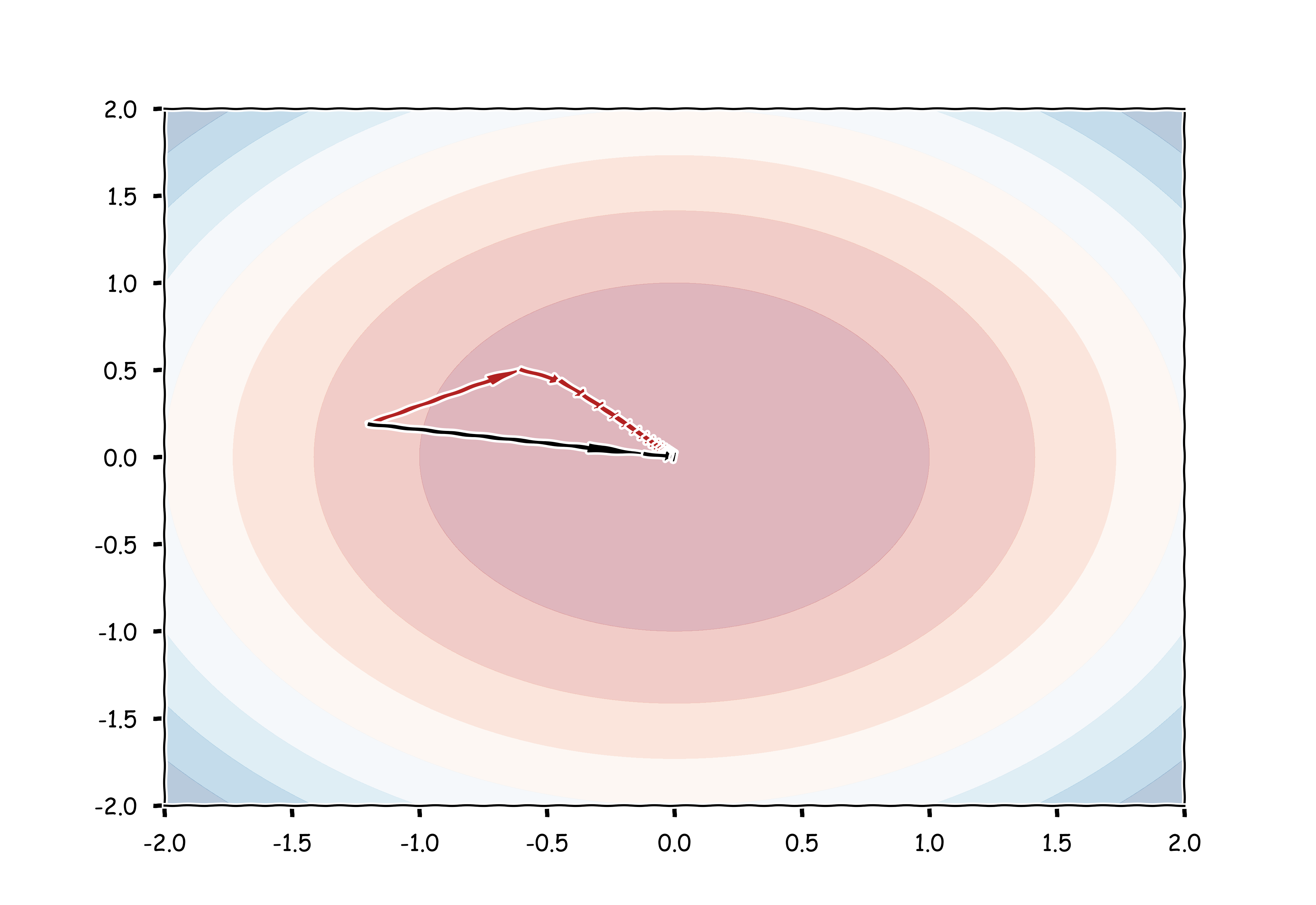Eigenvalues of iterates of Gradient Descent on $\hat{h}$ with correct (black) and incorrect (red) gradients

As we can clearly see, working with the incorrect understanding of gradients can leads to suboptimal convergence in iterative algorithms like gradient descent. Hopefully this little factoid made this long read worthwhile.